Enter your data
Pick a table — XY for curves, Column for comparing groups, Grouped for two factors, Contingency for counts — then type, paste from a spreadsheet or import a CSV or .xlsx file.
Paste your data, fit dose–response, enzyme kinetics, exponential or your own equation, and get each parameter with its standard error, 95% confidence interval and the goodness of fit.
Run t tests, ANOVA with multiple comparisons, nonparametric and chi-square tests, then save the graph as SVG, PNG or PDF.
Loading the workspace…
Pick a table — XY for curves, Column for comparing groups, Grouped for two factors, Contingency for counts — then type, paste from a spreadsheet or import a CSV or .xlsx file.
Pick an equation or a test. Results update as you edit: parameters with confidence intervals, P values with stars and a plain-language summary.
Adjust error bars, axes, fonts and colours, show the fitted curve or significance brackets, and save it as SVG, PNG (up to 1200 dpi) or PDF.
Lines and polynomials, one- and two-phase exponential decay and association, growth, power, logarithmic, Michaelis–Menten, Hill, Gaussian, Boltzmann — or type your own equation. Starting values are found for you.
Four- and five-parameter logistic fits give the IC50/EC50 with its confidence interval. Type unknown Y values to read concentrations off a standard curve.
Standard errors and 95% confidence intervals of every parameter, R², adjusted R², Sy.x, RMSE, AICc, the runs test and a residual plot. Compare two equations by F test and AICc.
Unpaired, Welch and paired t tests, Mann–Whitney and Wilcoxon, one-way ANOVA with Tukey, Bonferroni or Dunnett, Kruskal–Wallis with Dunn, and two-way ANOVA. Also from mean, SD and N.
Descriptive statistics, Shapiro–Wilk and D’Agostino normality tests, Grubbs’ outlier test, Pearson and Spearman correlation, chi-square and Fisher’s exact test with odds ratio and relative risk.
Scatter with fitted curves and confidence bands, bar, dot, box and violin plots, error bars, significance brackets, log axes. Vector SVG and PDF with embedded fonts, PNG at print resolution.
Dose–response equations use log(dose) as X. If your X column holds concentrations, tick “X values are concentrations” — points at zero concentration are left out.
If the response must start at 0 or end at 100%, open Constraints and fix Bottom or Top. Fewer free parameters give tighter confidence intervals.
For paired t and Wilcoxon tests, keep each subject’s two values on the same row of the Column table.
SD shows how spread the values are; SEM how precisely the mean is known. Say which one your error bars show in the legend of your figure.
Copy puts the result tables on the clipboard ready to paste into a spreadsheet or document; CSV saves them as a file.
Write Y = Bottom + (Top − Bottom)/(1 + exp((V50 − x)/Slope)). Any name other than x becomes a parameter; log is base 10, ln is natural.
Make illustrations, cover images and short clips with WaveSpeed AI.
Create diagrams-style illustrations and cover art for slides and posters.
Turn a still into a short clip for a talk or social post.
Turn a picture into a 3D model.
$1 in free credits for eligible new accounts. No card needed. Generators have separate account and credit requirements. The curve fitting tool is free.
Yes. No account, no watermark on graphs, no limit on fits or tests, and no paid tier.
No. Every calculation runs in your browser tab. The page only downloads the open fonts it draws graph text with; your values are never sent anywhere. The project is saved in this browser only.
The fitting engine reproduces the certified values of all 27 NIST StRD nonlinear regression reference problems — best-fit parameters to at least 6 significant digits from NIST’s second starting values. From NIST’s first, deliberately poor starting values, two of the hardest problems (BoxBOD and MGH10) stop at a different minimum, as in most fitting programs. Every test and fit is also checked against widely used open-source scientific libraries.
Put log(concentration) in the X column (or concentrations, and tick “X values are concentrations”), the responses in Y, and choose “log(dose) vs response, 4 parameters”. The result shows LogEC50 and the EC50/IC50 with its 95% confidence interval. For an inhibition curve the Hill slope is negative.
Descriptive statistics; unpaired, Welch and paired t tests; one-sample t and Wilcoxon tests; Mann–Whitney; Wilcoxon matched pairs; one-way ANOVA with Tukey, Bonferroni or Dunnett, Welch’s ANOVA, Bartlett and Brown–Forsythe; Kruskal–Wallis with Dunn; two-way ANOVA with comparisons within rows; Pearson and Spearman correlation; chi-square and Fisher’s exact test; Shapiro–Wilk and D’Agostino–Pearson; Grubbs’ outlier test.
Yes. Select cells in your spreadsheet, copy, click a cell in the table and press Ctrl+V (Cmd+V on a Mac). Decimal commas are understood. You can also import CSV, TSV and .xlsx files.
It has no repeated-measures ANOVA, no global fitting with parameters shared between data sets, Fisher’s exact test only for 2×2 tables, no ROUT outlier method and no survival analysis. Two-way ANOVA needs individual replicate values. Very large Dunnett comparisons (dozens of groups) take a few seconds.
None (ordinary least squares), relative 1/Y² using each point’s Y value, or 1/SD² using the SD of each X’s replicates or your SD column. Weighted fits report weighted sums of squares and R².
SVG and PDF are vector files: lines and text stay sharp at any size, and the PDF embeds its fonts. PNG goes up to 1200 dpi and records its resolution. Fonts have the same widths as Arial and Times New Roman.
Paste values, pick an equation or a test, and export the graph.
/filters:quality(82)/media/images/1791123751656780930_IfFPY7R0.webp)
/filters:quality(82)/media/images/1791123737177812425_RjKT3cku.webp)
/filters:quality(82)/media/images/1791123748309870128_xlkNgK8N.webp)
/filters:quality(82)/media/images/1791123738630744263_oR09R0aj.webp)
/filters:quality(82)/media/images/1791177033162457776_uQ09OY7g.webp)
/filters:quality(82)/media/images/1791123734319125607_JdnwGPY7.webp)
/filters:quality(82)/media/images/1791123746355630206_udnxGPY7.webp)
/filters:quality(82)/media/images/1791123744771362580_yC0sPezZ.webp)
/filters:quality(82)/media/images/1791123738606970169_5KIR1ais.webp)
/filters:quality(82)/media/images/1791123748197655725_EUmuFNW6.webp)